Are you already tired of searching for the solution to the question: “How to remove duplicates in Excel?” I think, if you are going to work with a lot of data in your spreadsheets, you know that it is a big headache when you have multiple duplicates among the rows. Not only it confuses you, but also wastes a lot of time when trying to analyze a situation. So, in this article I will tell you how it is possible to find and remove duplicates from Excel.
Duplicates play a great role in data analysis process. When you have duplicate data, it means that you have more than one record of same values for different fields. The duplicates may be occurring due to manual errors or multiple records from the same source. Duplicate records are just a part of business and there’s nothing to be worried about. Being a mixed bag, duplicating is also good in some cases when introduced deliberately in order to ensure accurate data entry. So, what happens when dealing with duplicates helps in data analysis? You get only the one which represents the most accurate information.
Table of Contents
Find And Remove Duplicate Values With The Remove Duplicates Command
Excel has a built-in tool that helps delete repeated entries in your dataset. Let’s have a look at the steps to be followed to remove duplicates in Excel.
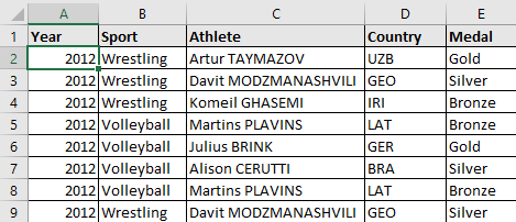
- First, click on any cell or a specific range in the dataset from which you want to remove duplicates. If you click on a single cell, Excel automatically determines the range for you in the next step.
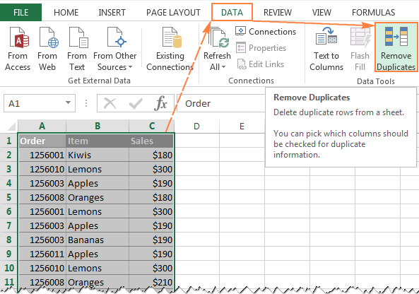
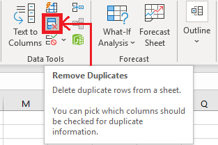
- Next, locate the ‘Remove Duplicates’ option and select it.
DATA tab → Data Tools section → Remove Duplicates
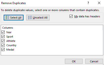
- A dialog box appears, as shown below. You can select the columns you want to compare and check for duplicate data.
In case your data consists of column headers, select the ‘My data has headers’ option, and then click on OK.
Post Graduate Program in Business Analysis
In partnership with Purdue UniversityVIEW COURSE
On checking the header option, the first row will not be considered for removing duplicate values.
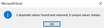
- Excel will now delete the duplicate rows and display a dialog box. The dialog box shows a summary of how many duplicate values are found and removed along with the count of unique values.
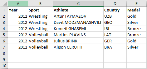
- As you can notice, the duplicate records are removed.
Find And Remove Duplicate Values With Advanced Filters
There is also another way to get rid of any duplicate values in your data from the ribbon. This is possible from the advanced filters.
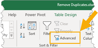
Select a cell inside the data and go to the Data tab and click on the Advanced filter command.
This will open up the Advanced Filter window.
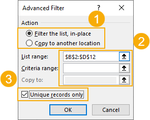
- You can choose to either to Filter the list in place or Copy to another location. Filtering the list in place will hide rows containing any duplicates while copying to another location will create a copy of the data.
- Excel will guess the range of data, but you can adjust it in the List range. The Criteria range can be left blank and the Copy to field will need to be filled if the Copy to another location option was chosen.
- Check the box for Unique records only.
Press OK and you will eliminate the duplicate values.
Advanced filters can be a handy option for getting rid of your duplicate values and creating a copy of your data at the same time. But advanced filters will only be able to perform this on the entire table.
Find And Remove Duplicate Values With A Pivot Table
Pivot tables are just for analyzing your data, right?
You can actually use them to remove duplicate data as well!
You won’t actually be removing duplicate values from your data with this method, you will be using a pivot table to display only the unique values from the data set.
First, create a pivot table based on your data. Select a cell inside your data or the entire range of data ➜ go to the Insert tab ➜ select PivotTable ➜ press OK in the Create PivotTable dialog box.
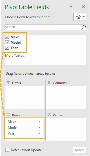
With the new blank pivot table add all fields into the Rows area of the pivot table.
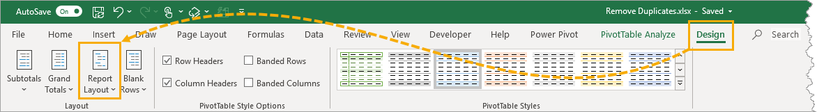
You will then need to change the layout of the resulting pivot table so it’s in a tabular format. With the pivot table selected, go to the Design tab and select Report Layout. There are two options you will need to change here.
- Select the Show in Tabular Form option.
- Select the Repeat All Item Labels option.
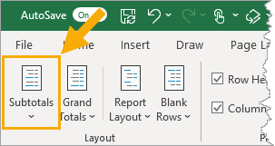
You will also need to remove any subtotals from the pivot table. Go to the Design tab ➜ select Subtotals ➜ select Do Not Show Subtotals.
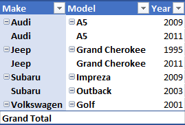
You now have a pivot table that mimics a tabular set of data!
Pivot tables only list unique values for items in the Rows area, so this pivot table will automatically remove any duplicates in your data.
Find And Remove Duplicate Values With Power Query
Power Query is all about data transformation, so you can be sure it has the ability to find and remove duplicate values.
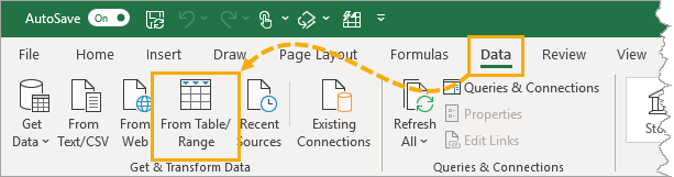
Select the table of values which you want to remove duplicates from ➜ go to the Data tab ➜ choose a From Table/Range query.
Remove Duplicates Based On One Or More Columns
With Power Query, you can remove duplicates based on one or more columns in the table.
You need to select which columns to remove duplicates based on. You can hold Ctrl to select multiple columns.
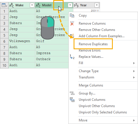
Right click on the selected column heading and choose Remove Duplicates from the menu.
You can also access this command from the Home tab ➜ Remove Rows ➜ Remove Duplicates.
= Table.Distinct(#"Previous Step", {"Make", "Model"})If you look at the formula that’s created, it is using the Table.Distinct function with the second parameter referencing which columns to use.
Remove Duplicates Based On The Entire Table
To remove duplicates based on the entire table, you could select all the columns in the table then remove duplicates. But there is a faster method that doesn’t require selecting all the columns.
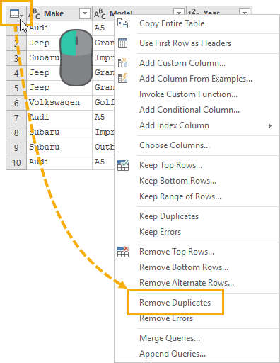
There is a button in the top left corner of the data preview with a selection of commands that can be applied to the entire table.
Click on the table button in the top left corner ➜ then choose Remove Duplicates.
= Table.Distinct(#"Previous Step")If you look at the formula that’s created, it uses the same Table.Distinct function with no second parameter. Without the second parameter, the function will act on the whole table.
Keep Duplicates Based On A Single Column Or On The Entire Table
In Power Query, there are also commands for keeping duplicates for selected columns or for the entire table.
Follow the same steps as removing duplicates, but use the Keep Rows ➜ Keep Duplicates command instead. This will show you all the data that has a duplicate value.
Find And Remove Duplicate Values Using A Formula
You can use a formula to help you find duplicate values in your data. https://7438b5a1c0fb643ba35e58f429534360.safeframe.googlesyndication.com/safeframe/1-0-38/html/container.html

First you will need to add a helper column that combines the data from any columns which you want to base your duplicate definition on.
= [@Make] & [@Model] & [@Year]The above formula will concatenate all three columns into a single column. It uses the ampersand operator to join each column.
= TEXTJOIN("", FALSE , CarList[@[Make]:[Year]])If you have a long list of columns to combine, you can use the above formula instead. This way you can simply reference all the columns as a single range.
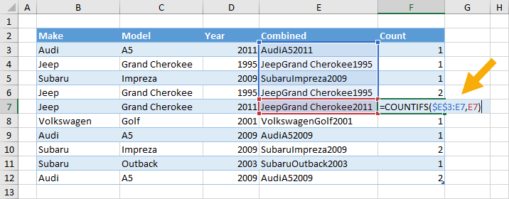
You will then need to add another column to count the duplicate values. This will be used later to filter out rows of data that appear more than once.
= COUNTIFS($E$3:E3, E3)Copy the above formula down the column and it will count the number of times the current value appears in the list of values above.
If the count is 1 then it’s the first time the value is appearing in the data and you will keep this in your set of unique values. If the count is 2 or more then the value has already appeared in the data and it is a duplicate value which can be removed.
Add filters to your data list.
- Go to the Data tab and select the Filter command.
- Use the keyboard shortcut Ctrl + Shift + L.
Now you can filter on the Count column. Filtering on 1 will produce all the unique values and remove any duplicates.
You can then select the visible cells from the resulting filter to copy and paste elsewhere. Use the keyboard shortcut Alt + ; to select only the visible cells.
Find And Remove Duplicate Values With Conditional Formatting
With conditional formatting, there’s a way to highlight duplicate values in your data.
Just like the formula method, you need to add a helper column that combines the data from columns. The conditional formatting doesn’t work with data across rows, so you’ll need this combined column if you want to detect duplicates based on more than one column.
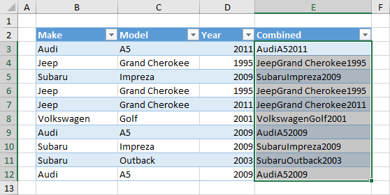
Then you need to select the column of combined data.
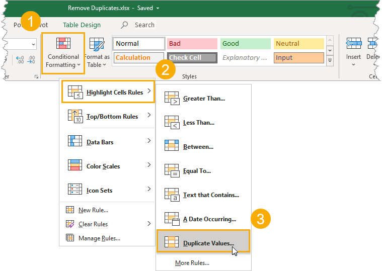
To create the conditional formatting, go to the Home tab ➜ select Conditional Formatting ➜ Highlight Cells Rules ➜ Duplicate Values.
This will open up the conditional formatting Duplicate Values window.
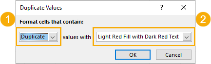
- You can select to either highlight Duplicate or Unique values.
- You can also choose from a selection of predefined cell formats to highlight the values or create your own custom format.
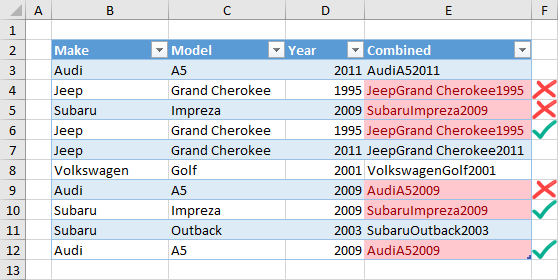
Warning: The previous methods to find and remove duplicates considers the first occurrence of a value as a duplicate and will leave it intact. However, this method will highlight the first occurrence and will not make any distinction.
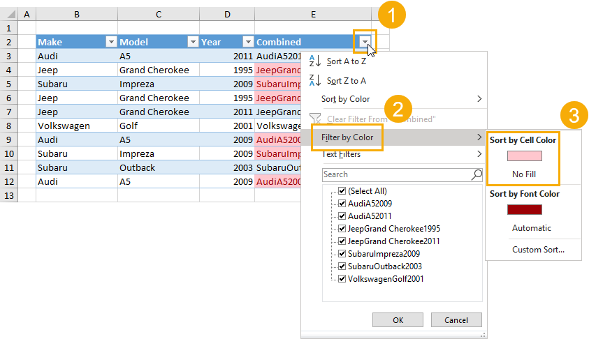
With the values highlighted, you can now filter on either the duplicate or unique values with the filter by color option. Make sure to add filters to your data. Go to the Data tab and select the Filter command or use the keyboard shortcut Ctrl + Shift + L.
- Click on the filter toggle.
- Select Filter by Color in the menu.
- Filter on the color used in the conditional formatting to select duplicate values or filter on No Fill to select unique values.
You can then select just the visible cells with the keyboard shortcut Alt + ;.
Find And Remove Duplicate Values Using VBA
There is a built in command in VBA for removing duplicates within list objects.
Sub RemoveDuplicates()Dim DuplicateValues As RangeSet DuplicateValues = ActiveSheet.ListObjects("CarList").RangeDuplicateValues.RemoveDuplicates Columns:=Array(1, 2, 3), Header:=xlYesEnd Sub
The above procedure will remove duplicates from an Excel table named CarList.
Columns:=Array(1, 2, 3)The above part of the procedure will set which columns to base duplicate detection on. In this case it will be on the entire table since all three columns are listed.
Header:=xlYesThe above part of the procedure tells Excel the first row in our list contains column headings.
You will want to create a copy of your data before running this VBA code, as it can’t be undone after the code runs.
Conclusion
Duplicate data may occur in your excel file for various reasons. It can happen accidentally if you copy and paste data from one cell to another or duplicate you data by entering the same information multiple times. It is also possible that this may happen as a result of merging sheets or copying text without adhere to adhere to copy paste options.