The How to Convert Text to Number in Excel article can help you convert text to value, including converting default text values to value, converting negative number into positive number, converting numeric data into text in Excel, and converting dates in excel.
It’s common to find numbers stored as text in Excel. This leads to incorrect calculations when you use these cells in Excel functions such as SUM and AVERAGE (as these functions ignore cells that have text values in it). In such cases, you need to convert cells that contain numbers as text back to numbers.
Now before we move forward, let’s first look at a few reasons why you may end up with a workbook that has numbers stored as text.
Table of Contents
How to Convert Text to Number in Excel
- Using ‘ (apostrophe) before a number.
- A lot of people enter apostrophe before a number to make it text. Sometimes, it’s also the case when you download data from a database. While this makes the numbers show up without the apostrophe, it impacts the cell by forcing it to treat the numbers as text.
- Getting numbers as a result of a formula (such as LEFT, RIGHT, or MID)
- If you extract the numerical part of a text string (or even a part of a number) using the TEXT functions, the result is a number in the text format.
Method 1: Using PC or Mac
- Open the Excel spreadsheet you want to edit. Find and double-click the spreadsheet file on your computer to open it in Microsoft Excel.
- Right-click the cell you want to edit. This will open your right-click options on a drop-down menu.
- Numbers formatted as text are left-aligned in a cell.
- If you want to change multiple cells, hold down ⌘ Command on Mac or Control on Windows, and click all the cells you want to edit. Then, right-click any of the selected cells.
- Click Format Cells on the right-click menu. This will open your cell formatting options in a new
- Select Number in the Category panel. You’ll find a list of all the available cell categories on the left-hand side of the Format Cells window. Click Number here to format the selected cells for numbers.
- Select the decimal places you want to use (optional). You can use the arrow keys next to the “Decimal places” counter or manually type the number of decimals you want use.
- All the selected cells will show the decimal places indicated here.
- Select a display format for negative numbers (optional). You can select how you’re going to see negative numbers in the “Negative numbers” box. It’s at the bottom of the Format Cells window.
- Click OK. This button is in the lower-right corner of the Format Cells window. It will save and apply your new formatting to all the selected cells.
- Numbers in these cells should now be right-aligned, and properly processed in all formulas.
Method 2: Using iPhone, iPad or Android
- Open Excel on your phone or tablet. The Excel icon looks like a white spreadsheet icon and an “X” on a green background. You can find it on your home screen or on the Apps menu.
- Open the spreadsheet you want to edit. You can edit one of your saved spreadsheets or tap New on the bottom-left, and open a new spreadsheet.
- Tap the cell you want to edit. Tapping will select the cell, and show a green outline around it.
- Numbers formatted as text will look left-aligned in a cell.
- Tap the A icon at the top. This is your toolbar button on a navigation bar at the top of your screen. It looks like an “A” with a pencil on it. Tapping will open your toolbar options at the bottom.
- Scroll down and tap Number Format. This option is listed next to an “ABC 123” icon on the toolbar menu. It will open your cell formatting options.
- This option is found in your toolbar’s Home tab.
- If the toolbar opens up to a different tab, such as Insert, Formulas, Data or View, tap the tab’s name on the top-left of the menu, and select Home.
- Select Number on the Number Format menu. This will convert the selected cell to number format, and allow you to properly process the numbers in it in all formulas.
Convert Text to Numbers Using ‘Convert to Number’ Option
When an apostrophe is added to a number, it changes the number format to text format. In such cases, you’ll notice that there is a green triangle at the top left part of the cell.

In this case, you can easily convert numbers to text by following these steps:
- Select all the cells that you want to convert from text to numbers.

- Click on the yellow diamond shape icon that appears at the top right. From the menu that appears, select ‘Convert to Number’ option.
This would instantly convert all the numbers stored as text back to numbers. You would notice that the numbers get aligned to the right after the conversion (while these were aligned to the left when stored as text).
Convert Text to Numbers by Changing Cell Format
When the numbers are formatted as text, you can easily convert it back to numbers by changing the format of the cells.
Here are the steps:
- Select all the cells that you want to convert from text to numbers.
- Go to Home –> Number. In the Number Format drop-down, select General.
This would instantly change the format of the selected cells to General and the numbers would get aligned to the right. If you want, you can select any of the other formats (such as Number, Currency, Accounting) which will also lead to the value in cells being considered as numbers.
Convert Text to Numbers Using Paste Special Option
To convert text to numbers using Paste Special option:
- Enter 1 in any empty cell in the worksheet. Make sure it is formatted as a number (i.e., aligned to the right of the cell).
- Copy the cell that contains 1.
- Select the cells that you want to convert from text to numbers.
- Right-click and select Paste Special.

- In the Paste Special dialog box, select Multiply within the Operation category.

- Click OK.
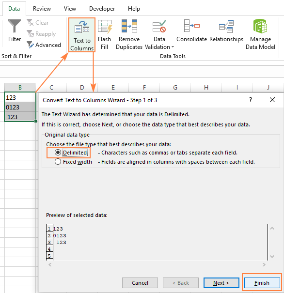
Convert Text to Numbers Using Text to Column
This method is suitable in cases where you have the data in a single column.
Here are the steps:
- Select all the cells that you want to convert from text to numbers.
- Go to Data –> Data Tools –> Text to Columns.

- In the Text to Column Wizard:
- In Step 1: Select Delimited and click on Next.

- In Step 2: Select Tab as the delimiter and click on Next.

- In Step 3: In Column data format, make sure General is selected. You can also specify the destination where you want the result. If you don’t specify anything, it will replace the original data set.

- In Step 1: Select Delimited and click on Next.
While you may still find the resulting cells to be in the text format, and the numbers still aligned to the left, now it would work in functions such as SUM and AVERAGE.
Conclusion
When working with Microsoft Excel, sometimes you may need to convert characters into numbers, or vice versa. You might even need to create or change that $ sign inside the cell so it displays with the number format you prefer.