How to Edit Legend in Excel – When a chart has a legend displayed, you can modify the individual legend entries by editing the corresponding data on the worksheet. For additional editing options, or to modify legend entries without affecting the worksheet data, you can make changes to the legend entries in the Select Data Source dialog box.
Table of Contents
How to show Excel legends on Chart
The main reason why a legend is in the Excel chart is to explain what type of data is being displayed in any of the colors. Legend contains a simple square that shows the descriptive text and the color. A good example is a chart that compares voter turnout for the last three voter seasons from 2000 in Kenya. The legend will show which color in the Chart stands for each of the general elections.
When you are creating a chart with that data, you are unlikely to see the legend displayed. What you are supposed to do is to fix this by selecting the entire Chart. After this, click on the plus sign button that you can check on the right of the Chart.
What follows here is to toggle on legends from the element menu. If you want to see the locations of the legend on the chart, you can click on the small black arrow in the Chart. With that in mind, let`s move to the other step.
Legends are automatically created for each chart you insert into your Excel workbooks. They’re the key to understanding how your chart reads and what information is depicted.
In charts with legends displayed, you may edit the individual legend entries on the worksheet by editing the corresponding data. Change the legend details in the Select Data Source dialog box for further customization options. This also ensures you can alter legend entries without influencing the worksheet data.
This article works for all software versions and platforms, however, we’ll be using the latest Microsoft Excel 2019 for Windows 10.
How to change legend entries in Excel
Below, you can find the current working methods of editing your chart legend in Excel, suitable for different approaches. Decide whether you want to alter your data, or simply want to modify the legend labels themselves, and proceed with the appropriate guide.
Need any help? Don’t hesitate to contact us for quick, expert assistance for all Microsoft Office products.
Method 1. Edit legend entries in your worksheet
If you want to modify the data cell as well as the legend that gets displayed on the chart, you can do so by editing the legend entry in your worksheet. To do this, follow the steps below.
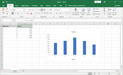
- Click the cell in your worksheet that contains the data that appears as an entry in the chart legend. In our example, the legend entry is “Sales” so we’ll be selecting the B1 cell:
- Start typing to modify the cell, and type in the new desired name for your legend entry. Press Enter on your keyboard when you’re done modifying the cell.
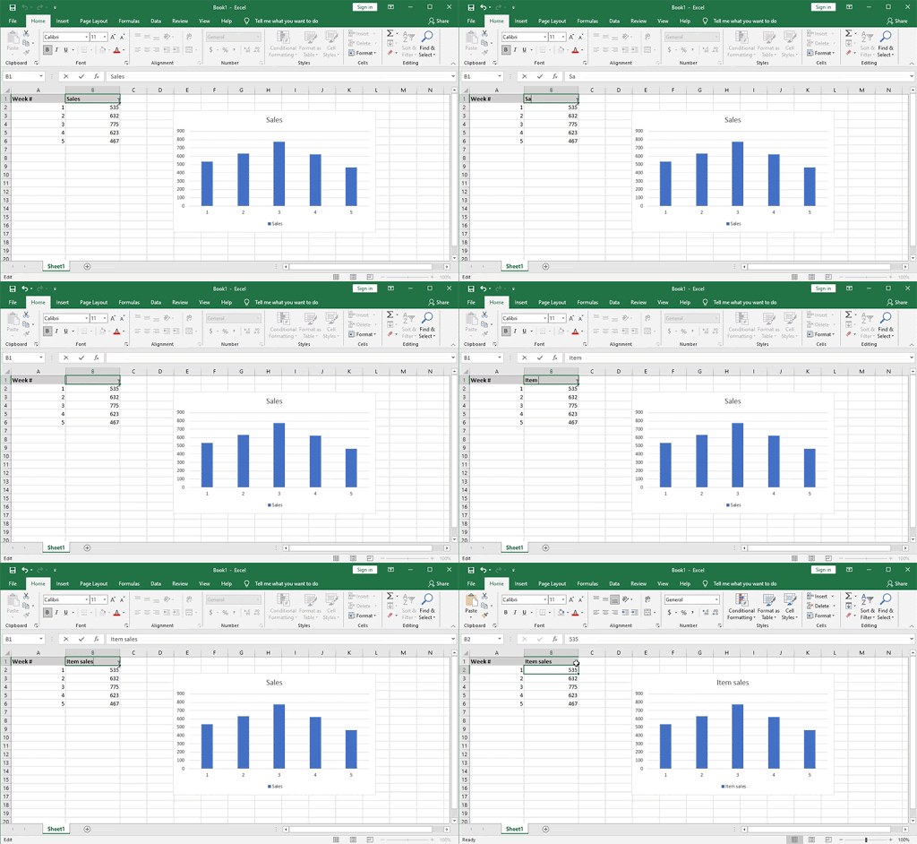
Imgur link - The change will automatically reflect in your chart, and the new legend name will appear in the legend on the chart.
Method 2. Use the Select Data Source feature
The alternative method of editing your chart legend is using a feature called Select Data Source. By following the steps below, you can alter the legend entry without having to modify the original cell in your worksheet.
- Select the chart you want to add a legend to. This should open some of the tabs in your ribbon interface which are hidden by default.
- Switch to the newly visible Design tab in your ribbon interface. Click on the Select Data button from the Data group.

- A new pop-up window should appear. Here, look for a box called Legend Entries (Series) and then select the legend you want to modify. In our example, we’ll be editing the “Sales” legend.
- Click on the Edit button.
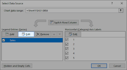
- Use the Series Name input box to do one of the following:
- Type the legend entry name that you want to use. This will be a static name that you need to change manually, even if the original cell is altered.
- Type the reference to the worksheet cell that contains the data that you want to use as the legend name. This is dynamic, meaning that you only need to modify the cell name to reflect changes in the chart.
- Press Enter after editing the legend entry. Click OK to close the Select Data Source window.
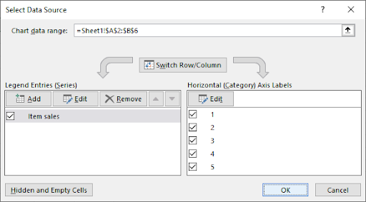
- Done!
How to change legend position?
It is very easy to change the legend position in Excel. Simply click the chart, then click the Layout tab. Under Legend, choose the preferred position from the drop-down menu.
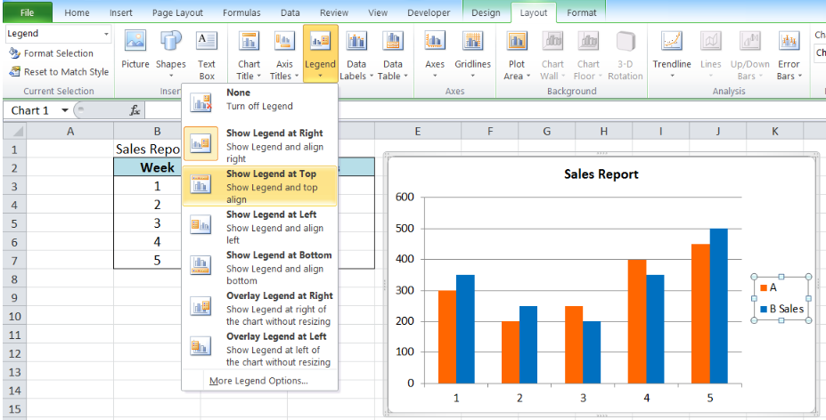
Figure 11. Change legend position
Example:
Select Show Legend at Top from the drop-down menu. As shown below, the legend is transferred to the top of the chart.

Figure 12. Output: Change legend position
How to edit legend format?
In order to change the format, right-click the legend and select Format Legend.

Figure 13. Edit legend through Format Legend
The Format Legend dialog box will appear. There are several options where we can change the legend position, fill, border color, border styles, and other formatting options.

Figure 14. Format legend preview pane
Example:
We want to fill the legend box with Aqua, Accent 5, Lighter 60%.
We click Fill, then tick Solid Fill.

Figure 15. Change legend fill
Choose the color we prefer and click OK. The fill color will automatically be updated to the chosen color.

Figure 16. Select fill color for legend
We can add more formatting changes. Below chart shows the legend format with a 5% pattern fill and an orange border color.

Conclusion
We hope that this article helped you learn how to edit a legend in Excel and modify chart legends. Now, you can keep your charts dynamic and up-to-date with your data, no matter how many changes are made.
