When you create different types of data tables in Excel, it automatically applies table formatting to the data. If you want to showcase your data in a clear and organized manner, removing this table formatting is an option. You can remove it by following simple steps discussed below. Even though you don’t have much control over table formats in Excel, you can put them to work for you too, providing you with enough space to perform different types of calculations on data.
Keep reading this article to learn How to Remove Table Formatting in Excel.
Table of Contents
Excel table styles
Excel tables make it a lot easier to view and manage data by providing a handful of special features such as integrated filter and sort options, calculated columns, structured references, total row, etc.
By converting data to an Excel table, you also get a head start on the formatting. A newly inserted table comes already formatted with font and background colors, banded rows, borders, and so on. If you don’t like the default table format, you can easily change it by selecting any of the inbuilt Table Styles on the Design tab.
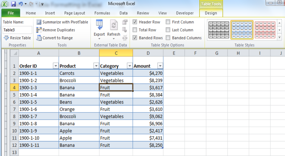
The Design tab is the starting point to work with Excel table styles. It appears under the Table Tools contextual tab, as soon as you click any cell within a table.

As you can see on the screenshot above, the Table Styles gallery provides a collection of 50+ inbuilt styles grouped into Light, Medium, and Dark categories.
You can think of an Excel table style as a formatting template that automatically applies certain formats to table rows and columns, headers and totals row.
Apart from table formatting, you can use the Table Style Options to format the following table elements:
- Header row – display or hide the table headers.
- Total row – add the totals row at the end of the table with a list of functions for each total row cell.
- Banded rows and banded columns – show alternate row or column shading, respectively.
- First column and last column – apply special formatting for the first and last column of the table.
- Filter button – display or hide the filter arrows in the header row.
The following screenshot demonstrates the default Table Style options:
How to Remove Excel Table Formatting (while keeping the Table)
Suppose I have the dataset as shown below.

When I covert this data into an Excel table (keyboard shortcut Control + T), I get something as shown below.

You can see that Excel has gone ahead and applied some formatting to the table (apart from adding filters).
In most cases, I don’t like the formatting Excel automatically applies and I need to change this.
I can now remove the formatting from the table completely or I can modify it to look the way I want.
Let me show you how to do both.
Remove Formatting from the Excel Table
Below are the steps to remove the Excel table formatting:
- Select any cell in the Excel table
- Click the Design tab (this is a contextual tab and only appears when you click any cell in the table)

- In Table Styles, click on the More icon (the one at the bottom of the small scrollbar

- Click on the Clear option.

The above steps would remove the Excel Table formatting, while still keeping it as a table. You will still see the filters that are automatically added, just the formatting has been removed.
You can now format it manually if you want.
Change the Formatting of the Excel Table
If you don’t like the default formatting applied to an Excel Table, you can also modify it by choosing from some presets.
Suppose you have the Excel table and shown below and you want to modify the formatting of this.
Below are the steps to do this:
- Select any cell in the Excel table
- Click the Design tab (this is a contextual tab and only appears when you click any cell in the table)
- In Table Styles, click on the More icon (the one at the bottom of the small scrollbar
- Choose from any of the existing designs

When you hover your cursor over any design, you will be able to see the live preview of how that formatting will look in your Excel Table. Once you have finalized the formatting you want, simply click on it.
In case you don’t like any of the existing Excel table styles, you can also create your own format by clicking on the ‘New Table Styles’. This will open a dialog box where you can set the formatting.
Remove Excel Table (Convert to Range) & the Formatting
It’s easy to convert tabular data into an Excel table, and it’s equally easy to convert an Excel table back to the regular range.
But the thing that can be a bit frustrating is that when you convert an Excel table to the range, it leaves the formatting behind.
And now you have to manually clear the Excel table formatting.
Suppose you have the Excel table as shown below:
Below are the steps to convert this Excel table to a range:
- Right-click on any cell in the Excel table
- Go to the Table option
- Click on ‘Convert to Range’

This will give you a result as shown below (where the table has been deleted but the formatting remains).
Now you can manually change the formatting or you can delete all the formatting altogether.
To remove all the formatting, follow the below steps:
- Select the entire range that has the formatting
- Click the Home tab
- In the Editing group, click on Clear
- In the options that show up, click on Clear Formats
This would leave you with only the data and all the formatting would be removed.
Another way of doing this could be to first remove all the formatting from the Excel Table itself (method covered in the previous section), and then delete the table (Convert to Range).
Delete the Table
This one is easy.
If you want to get rid of the table altogether, follow the below steps:
- Select the entire table
- Hit the Delete key
This will delete the Excel table and also remove any formatting it has (except the formatting that you have applied manually).
In case you have some formatting applied manually that you also want to remove while deleting the table, follow the below steps:
- Select the entire Excel table
- Click the Home tab

- Click on Clear (in Editing group)

- Click on Clear All

Keyboard shortcut to clear all in Excel Windows is ALT + H + E + A (press these keys one after the other in succession).
So these are some scenarios where you can remove table formatting in Excel.
Conclusion
Table formatting is an important part of Excel worksheet. You can modify the maximum number of rows and columns, resize the columns, control the border style for cells, control whether alternating row colors are used, control the alignment of text in cells, control cell background color among others. If you have to apply table formatting in your Excel spreadsheet, you have many options to choose from to format data.